Data Accession
For today’s workshop we will be using the pandas library, the
matplotlib library, and the seaborn library. Also, we will read
data from the web with the pandas-datareader. By the end of the
workshop, participants should be able to use Python to tell a story
about a dataset they build from an open data source.
GOALS:
- Understand how to load data as
.csvfiles into Pandas - Import data from web with
pandas-datareaderand compare development indicators from the World Bank - Use API’s and requests to pull data from web
.csv files
In the first session, we explored built-in datasets. Typically, we would
want to use our own data for analysis. A common filetype is the .csv
or comma separated values type. You have probably used a spreadsheet
program before, something like Microsoft Excel or Google Sheets. These
programs allow you to save the data as a universally recognized formats,
including the .csv extension. This is important as the .csv
filetype can be understood and read by most data analysis languages
including Python and R.
To begin, we will use Python to load a .csv file. Starting with the
tips dataset from last lesson, we will save this data as a csv file in
our data folder. Then, we can read the data in using Pandas read_csv
method.
In [1]:
%matplotlib notebook
import matplotlib.pyplot as plt
import numpy as np
import pandas as pd
import seaborn as sns
In [2]:
tips = sns.load_dataset("tips")
In [3]:
tips.head()
Out[3]:
| total_bill | tip | sex | smoker | day | time | size | |
|---|---|---|---|---|---|---|---|
| 0 | 16.99 | 1.01 | Female | No | Sun | Dinner | 2 |
| 1 | 10.34 | 1.66 | Male | No | Sun | Dinner | 3 |
| 2 | 21.01 | 3.50 | Male | No | Sun | Dinner | 3 |
| 3 | 23.68 | 3.31 | Male | No | Sun | Dinner | 2 |
| 4 | 24.59 | 3.61 | Female | No | Sun | Dinner | 4 |
In [4]:
tips.to_csv('data/tips.csv')
In [5]:
tips = pd.read_csv('data/tips.csv')
In [6]:
tips.head()
Out[6]:
| Unnamed: 0 | total_bill | tip | sex | smoker | day | time | size | |
|---|---|---|---|---|---|---|---|---|
| 0 | 0 | 16.99 | 1.01 | Female | No | Sun | Dinner | 2 |
| 1 | 1 | 10.34 | 1.66 | Male | No | Sun | Dinner | 3 |
| 2 | 2 | 21.01 | 3.50 | Male | No | Sun | Dinner | 3 |
| 3 | 3 | 23.68 | 3.31 | Male | No | Sun | Dinner | 2 |
| 4 | 4 | 24.59 | 3.61 | Female | No | Sun | Dinner | 4 |
In [13]:
# add a column for tip percent
tips['tip_pct'] = tips['tip']/tips['total_bill']
In [14]:
# create variable grouped that groups the tips by sex and smoker
grouped = tips.groupby(['sex', 'smoker'])
In [15]:
# create variable grouped_pct that contains the tip_pct column from grouped
grouped_pct = grouped['tip_pct']
In [16]:
#what does executing this cell show?  Explain the .agg method.
grouped_pct.agg('mean')
Out[16]:
sex     smoker
Female  No        0.156921
        Yes       0.182150
Male    No        0.160669
        Yes       0.152771
Name: tip_pct, dtype: float64
In [19]:
# What other options can you pass to the .agg function?
grouped_pct.agg(['mean', 'std'])
Out[19]:
| mean | std | ||
|---|---|---|---|
| sex | smoker | ||
| Female | No | 0.156921 | 0.036421 |
| Yes | 0.182150 | 0.071595 | |
| Male | No | 0.160669 | 0.041849 |
| Yes | 0.152771 | 0.090588 |
In [20]:
grouped_pct.agg?
Reading .csv files from web
If we have access to the file as a url, we can use the Pandas
read_csv method to pass the url of the csv file instead of loading
it from our local machine. For example, the Data and Software Carpentry
organizations have a .csv file located in their github repository as
seen below.
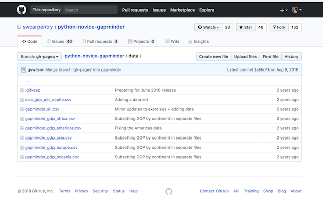
The first file on asia_gdp_per_capita can be loaded by using the
link to the raw file on github:
hence, we pass this url to the read_csv function and have a new
dataframe.
In [7]:
asia_gdp = pd.read_csv('https://raw.githubusercontent.com/swcarpentry/python-novice-gapminder/gh-pages/data/asia_gdp_per_capita.csv')
In [8]:
asia_gdp.head()
Out[8]:
| 'year' | 'Afghanistan' | 'Bahrain' | 'Bangladesh' | 'Cambodia' | 'China' | 'Hong Kong China' | 'India' | 'Indonesia' | 'Iran' | ... | 'Philippines' | 'Saudi Arabia' | 'Singapore' | 'Sri Lanka' | 'Syria' | 'Taiwan' | 'Thailand' | 'Vietnam' | 'West Bank and Gaza' | 'Yemen Rep.' | |
|---|---|---|---|---|---|---|---|---|---|---|---|---|---|---|---|---|---|---|---|---|---|
| 0 | 1952 | 779.445314 | 9867.084765 | 684.244172 | 368.469286 | 400.448611 | 3054.421209 | 546.565749 | 749.681655 | 3035.326002 | ... | 1272.880995 | 6459.554823 | 2315.138227 | 1083.532030 | 1643.485354 | 1206.947913 | 757.797418 | 605.066492 | 1515.592329 | 781.717576 |
| 1 | 1957 | 820.853030 | 11635.799450 | 661.637458 | 434.038336 | 575.987001 | 3629.076457 | 590.061996 | 858.900271 | 3290.257643 | ... | 1547.944844 | 8157.591248 | 2843.104409 | 1072.546602 | 2117.234893 | 1507.861290 | 793.577415 | 676.285448 | 1827.067742 | 804.830455 |
| 2 | 1962 | 853.100710 | 12753.275140 | 686.341554 | 496.913648 | 487.674018 | 4692.648272 | 658.347151 | 849.289770 | 4187.329802 | ... | 1649.552153 | 11626.419750 | 3674.735572 | 1074.471960 | 2193.037133 | 1822.879028 | 1002.199172 | 772.049160 | 2198.956312 | 825.623201 |
| 3 | 1967 | 836.197138 | 14804.672700 | 721.186086 | 523.432314 | 612.705693 | 6197.962814 | 700.770611 | 762.431772 | 5906.731805 | ... | 1814.127430 | 16903.048860 | 4977.418540 | 1135.514326 | 1881.923632 | 2643.858681 | 1295.460660 | 637.123289 | 2649.715007 | 862.442146 |
| 4 | 1972 | 739.981106 | 18268.658390 | 630.233627 | 421.624026 | 676.900092 | 8315.928145 | 724.032527 | 1111.107907 | 9613.818607 | ... | 1989.374070 | 24837.428650 | 8597.756202 | 1213.395530 | 2571.423014 | 4062.523897 | 1524.358936 | 699.501644 | 3133.409277 | 1265.047031 |
5 rows × 34 columns
Problems
Try to locate and load some .csv files using the internet. There are
many great resources out there. Also, I want you to try the
pd.read_clipboard method, where you’ve copied a data table from the
internet. In both cases create a brief exploratory notebook for the data
that contains the following:
- Jupyter notebook with analysis and discussion
- Data folder with relevant
.csvfiles - Images folder with at least one image loaded into the notebook
Accessing data through API
Pandas has the functionality to access certain data through a
datareader. We will use the pandas_datareader to investigate
information about the World Bank. For more information, please see the
documentation:
http://pandas-datareader.readthedocs.io/en/latest/remote_data.html
We will explore other examples with the datareader later, but to start let’s access the World Bank’s data. For a full description of the available data, look over the source from the World Bank.
https://data.worldbank.org/indicator
In [38]:
from pandas_datareader import wb
In [39]:
import datetime
In [40]:
wb.search('gdp.*capita.*const').iloc[:,:2]
Out[40]:
| id | name | |
|---|---|---|
| 646 | 6.0.GDPpc_constant | GDP per capita, PPP (constant 2011 internation... |
| 8064 | NY.GDP.PCAP.KD | GDP per capita (constant 2010 US$) |
| 8066 | NY.GDP.PCAP.KN | GDP per capita (constant LCU) |
| 8068 | NY.GDP.PCAP.PP.KD | GDP per capita, PPP (constant 2011 internation... |
| 8069 | NY.GDP.PCAP.PP.KD.87 | GDP per capita, PPP (constant 1987 internation... |
In [41]:
dat = wb.download(indicator='NY.GDP.PCAP.KD', country=['US','CA','MX'], start = 2005, end = 2016)
In [43]:
dat['NY.GDP.PCAP.KD'].groupby(level=0).mean()
Out[43]:
country
Canada           48601.353408
Mexico            9236.997678
United States    49731.965366
Name: NY.GDP.PCAP.KD, dtype: float64
In [44]:
wb.search('cell.*%').iloc[:,:2]
Out[44]:
| id | name | |
|---|---|---|
| 6339 | IT.CEL.COVR.ZS | Population covered by mobile cellular network (%) |
| 6394 | IT.MOB.COV.ZS | Population coverage of mobile cellular telepho... |
In [45]:
ind = ['NY.GDP.PCAP.KD', 'IT.MOB.COV.ZS']
In [46]:
dat = wb.download(indicator=ind, country = 'all', start = 2011, end = 2011).dropna()
In [47]:
dat.columns = ['gdp', 'cellphone']
dat.tail()
Out[47]:
| gdp | cellphone | ||
|---|---|---|---|
| country | year | ||
| Swaziland | 2011 | 3704.140658 | 94.9 |
| Tunisia | 2011 | 4014.916793 | 100.0 |
| Uganda | 2011 | 629.240447 | 100.0 |
| Zambia | 2011 | 1499.728311 | 62.0 |
| Zimbabwe | 2011 | 813.834010 | 72.4 |
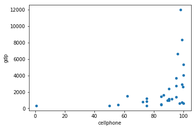
In [48]:
dat.plot(x ='cellphone', y = 'gdp', kind = 'scatter')
Out[48]:
<matplotlib.axes._subplots.AxesSubplot at 0x1a2215fe80>
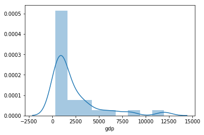
In [49]:
sns.distplot(dat['gdp']);
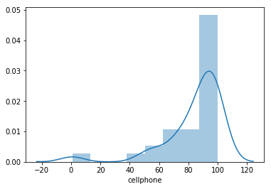
In [50]:
sns.distplot(dat['cellphone']);
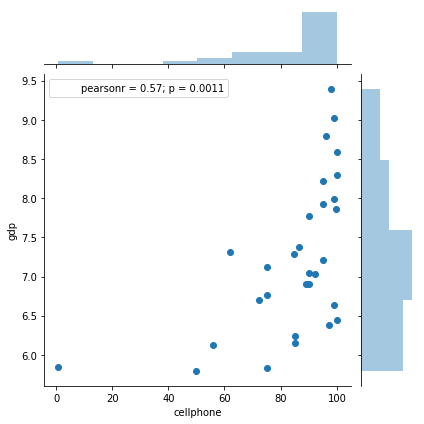
In [51]:
sns.jointplot(dat['cellphone'], np.log(dat['gdp']))
Out[51]:
<seaborn.axisgrid.JointGrid at 0x1a22099cf8>
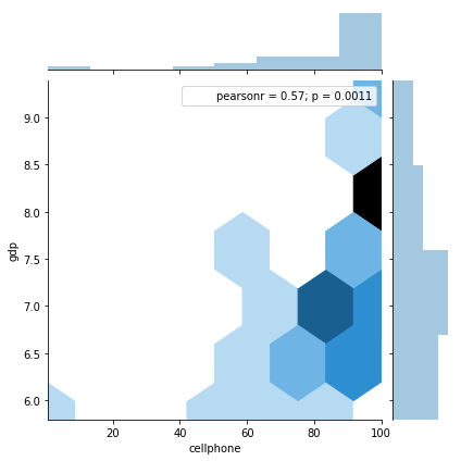
In [52]:
sns.jointplot(dat['cellphone'], np.log(dat['gdp']), kind = 'hex')
Out[52]:
<seaborn.axisgrid.JointGrid at 0x1a2144fc88>
StatsModels

StatsModels is a library that contains a wealth of classical statistical
techniques. Depending on your comfort or interest in deeper use of
classical statistics, you can consult the documentation at
http://www.statsmodels.org/stable/index.html . Below, we show how to use
statsmodels to perform a basic ordinary least squares fit with our
\(y\) or dependent variable as cellphone and \(x\) or
independent variable as log(gdp).
In [53]:
import numpy as np
import statsmodels.formula.api as smf
mod = smf.ols("cellphone ~ np.log(gdp)", dat).fit()
In [54]:
mod.summary()
Out[54]:
| Dep. Variable: | cellphone | R-squared: | 0.321 |
|---|---|---|---|
| Model: | OLS | Adj. R-squared: | 0.296 |
| Method: | Least Squares | F-statistic: | 13.21 |
| Date: | Sat, 13 Jan 2018 | Prob (F-statistic): | 0.00111 |
| Time: | 12:28:27 | Log-Likelihood: | -127.26 |
| No. Observations: | 30 | AIC: | 258.5 |
| Df Residuals: | 28 | BIC: | 261.3 |
| Df Model: | 1 | ||
| Covariance Type: | nonrobust |
| coef | std err | t | P>|t| | [0.025 | 0.975] | |
|---|---|---|---|---|---|---|
| Intercept | -2.3708 | 24.082 | -0.098 | 0.922 | -51.700 | 46.959 |
| np.log(gdp) | 11.9971 | 3.301 | 3.635 | 0.001 | 5.236 | 18.758 |
| Omnibus: | 27.737 | Durbin-Watson: | 2.064 |
|---|---|---|---|
| Prob(Omnibus): | 0.000 | Jarque-Bera (JB): | 62.978 |
| Skew: | -1.931 | Prob(JB): | 2.11e-14 |
| Kurtosis: | 8.956 | Cond. No. | 56.3 |