Decision Tree Classifiers
Example
Important Considerations
| PROS | CONS |
|---|---|
| Easy to visualize and Interpret | Prone to overfitting |
| No normalization of Data Necessary | Ensemble needed for better performance |
| Handles mixed feature types |
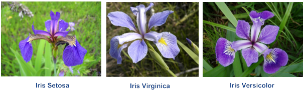
Iris Example
Use measurements to predict species
In [2]:
%matplotlib inline
import matplotlib.pyplot as plt
from sklearn.datasets import load_iris
from sklearn import tree
from sklearn.datasets import load_iris
from sklearn.tree import DecisionTreeClassifier
from sklearn.model_selection import train_test_split
In [3]:
import seaborn as sns
iris = sns.load_dataset('iris')
iris.head()
Out[3]:
| sepal_length | sepal_width | petal_length | petal_width | species | |
|---|---|---|---|---|---|
| 0 | 5.1 | 3.5 | 1.4 | 0.2 | setosa |
| 1 | 4.9 | 3.0 | 1.4 | 0.2 | setosa |
| 2 | 4.7 | 3.2 | 1.3 | 0.2 | setosa |
| 3 | 4.6 | 3.1 | 1.5 | 0.2 | setosa |
| 4 | 5.0 | 3.6 | 1.4 | 0.2 | setosa |
In [4]:
#split the data
iris = load_iris()
X_train, X_test, y_train, y_test = train_test_split(iris.data, iris.target)
In [5]:
len(X_test)
Out[5]:
38
In [6]:
#load classifier
clf = tree.DecisionTreeClassifier()
In [7]:
#fit train data
clf = clf.fit(X_train, y_train)
In [8]:
#examine score
clf.score(X_train, y_train)
Out[8]:
1.0
In [9]:
#against test set
clf.score(X_test, y_test)
Out[9]:
0.92105263157894735
How would specific flower be classified?
If we have a flower that has:
- Sepal.Length = 1.0
- Sepal.Width = 0.3
- Petal.Length = 1.4
- Petal.Width = 2.1
In [10]:
clf.predict_proba([[1.0, 0.3, 1.4, 2.1]])
Out[10]:
array([[ 0., 1., 0.]])
In [11]:
#cross validation
from sklearn.model_selection import cross_val_score
cross_val_score(clf, X_train, y_train, cv=10)
Out[11]:
array([ 0.83333333,  1.        ,  1.        ,  0.91666667,  0.91666667,
        1.        ,  0.90909091,  1.        ,  1.        ,  0.9       ])
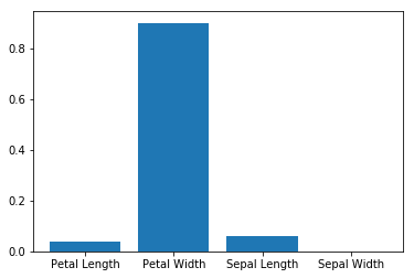
How important are different features?
In [12]:
#list of feature importance
clf.feature_importances_
Out[12]:
array([ 0.06184963, 0. , 0.03845214, 0.89969823])
In [13]:
imp = clf.feature_importances_
In [14]:
plt.bar(['Sepal Length', 'Sepal Width', 'Petal Length', 'Petal Width'], imp)
Out[14]:
<Container object of 4 artists>
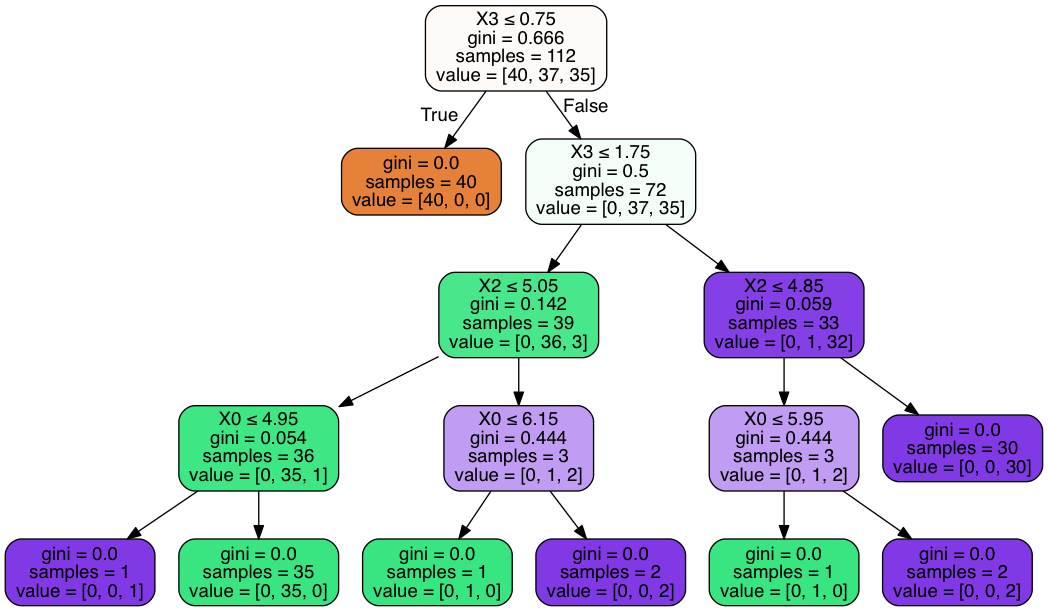
Visualizing Decision Tree
pip install pydotplus
In [15]:
from sklearn.externals.six import StringIO
from IPython.display import Image
from sklearn.tree import export_graphviz
import pydotplus

dot_data = StringIO()
export_graphviz(clf, out_file=dot_data,  filled=True, rounded=True, special_characters=True)
graph = pydotplus.graph_from_dot_data(dot_data.getvalue())
Image(graph.create_png())
Out[15]:
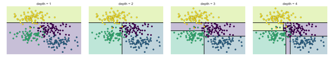
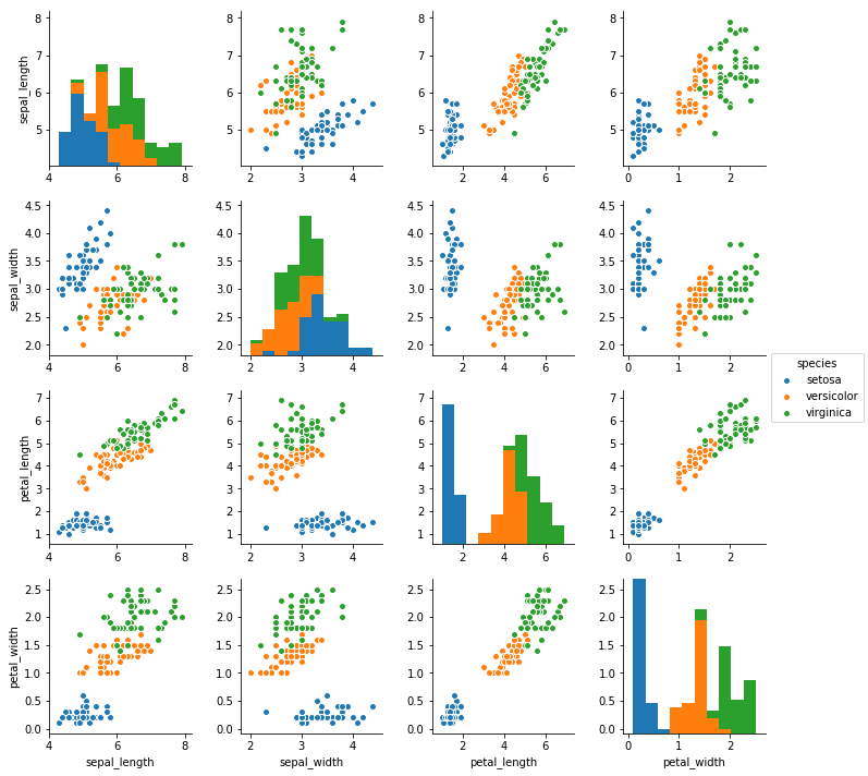
What’s Happening with Decision Tree
In [16]:
import seaborn as sns
iris = sns.load_dataset('iris')
sns.pairplot(data = iris, hue = 'species');
Pre-pruning: Avoiding Over-fitting
max_depth: limits depth of treemax_leaf_nodes: limits how many leafsmin_samples_leaf: limits splits to happen when only certain number of samples exist
In [17]:
clf = DecisionTreeClassifier(max_depth = 1).fit(X_train, y_train)
In [18]:
clf.score(X_train, y_train)
Out[18]:
0.6875
In [19]:
clf.score(X_test, y_test)
Out[19]:
0.60526315789473684
In [20]:
dot_data = StringIO()
export_graphviz(clf, out_file=dot_data,  filled=True, rounded=True, special_characters=True)
graph = pydotplus.graph_from_dot_data(dot_data.getvalue())
Image(graph.create_png())
Out[20]:
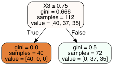
In [21]:
clf = DecisionTreeClassifier(max_depth = 2).fit(X_train, y_train)
In [22]:
clf.score(X_train, y_train)
Out[22]:
0.9642857142857143
In [23]:
clf.score(X_test, y_test)
Out[23]:
0.94736842105263153
In [24]:
dot_data = StringIO()
export_graphviz(clf, out_file=dot_data,  filled=True, rounded=True, special_characters=True)
graph = pydotplus.graph_from_dot_data(dot_data.getvalue())
Image(graph.create_png())
Out[24]:
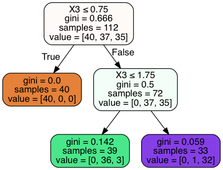
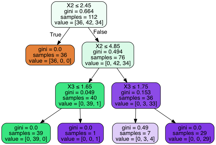
In [25]:
clf = DecisionTreeClassifier(max_depth = 3).fit(X_train, y_train)
clf.score(X_train, y_train)
Out[25]:
0.9732142857142857
In [26]:
clf.score(X_test, y_test)
Out[26]:
0.97368421052631582
Confusion Matrix
In [29]:
from sklearn.metrics import classification_report
import sklearn.metrics
from sklearn.metrics import confusion_matrix

classifier=clf.fit(X_train,y_train)

predictions=clf.predict(X_test)

mat = confusion_matrix(y_test, predictions)
sns.heatmap(mat.T, square=True, annot=True, fmt='d', cbar=False)
plt.xlabel('true label')
plt.ylabel('predicted label');
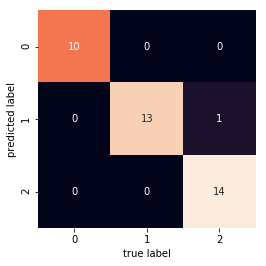
In [30]:
sklearn.metrics.confusion_matrix(y_test, predictions)
Out[30]:
array([[10,  0,  0],
       [ 0, 13,  0],
       [ 0,  1, 14]])
In [27]:
sklearn.metrics.accuracy_score(y_test, predictions)
Out[27]:
0.94736842105263153
In [28]:
dot_data2 = StringIO()
export_graphviz(clf, out_file=dot_data2,
                filled=True, rounded=True,
                special_characters=True)
graph2 = pydotplus.graph_from_dot_data(dot_data2.getvalue())
Image(graph2.create_png())
Out[28]:
In [29]:
sklearn.metrics.accuracy_score(y_test, predictions)
Out[29]:
0.94736842105263153
Example with Adolescent Health Data

In [33]:
from pandas import Series, DataFrame
import pandas as pd
import numpy as np
import matplotlib.pylab as plt

from sklearn.metrics import classification_report
import sklearn.metrics
In [34]:
AH_data = pd.read_csv("data/tree_addhealth.csv")
data_clean = AH_data.dropna()
data_clean.dtypes
Out[34]:
BIO_SEX      float64
HISPANIC     float64
WHITE        float64
BLACK        float64
NAMERICAN    float64
ASIAN        float64
age          float64
TREG1        float64
ALCEVR1      float64
ALCPROBS1      int64
marever1       int64
cocever1       int64
inhever1       int64
cigavail     float64
DEP1         float64
ESTEEM1      float64
VIOL1        float64
PASSIST        int64
DEVIANT1     float64
SCHCONN1     float64
GPA1         float64
EXPEL1       float64
FAMCONCT     float64
PARACTV      float64
PARPRES      float64
dtype: object
In [35]:
data_clean.describe()
Out[35]:
| BIO_SEX | HISPANIC | WHITE | BLACK | NAMERICAN | ASIAN | age | TREG1 | ALCEVR1 | ALCPROBS1 | ... | ESTEEM1 | VIOL1 | PASSIST | DEVIANT1 | SCHCONN1 | GPA1 | EXPEL1 | FAMCONCT | PARACTV | PARPRES | |
|---|---|---|---|---|---|---|---|---|---|---|---|---|---|---|---|---|---|---|---|---|---|
| count | 4575.000000 | 4575.000000 | 4575.000000 | 4575.000000 | 4575.000000 | 4575.000000 | 4575.000000 | 4575.000000 | 4575.000000 | 4575.000000 | ... | 4575.000000 | 4575.000000 | 4575.000000 | 4575.000000 | 4575.000000 | 4575.000000 | 4575.000000 | 4575.000000 | 4575.000000 | 4575.000000 |
| mean | 1.521093 | 0.111038 | 0.683279 | 0.236066 | 0.036284 | 0.040437 | 16.493052 | 0.176393 | 0.527432 | 0.369180 | ... | 40.952131 | 1.618579 | 0.102514 | 2.645027 | 28.360656 | 2.815647 | 0.040219 | 22.570557 | 6.290710 | 13.398033 |
| std | 0.499609 | 0.314214 | 0.465249 | 0.424709 | 0.187017 | 0.197004 | 1.552174 | 0.381196 | 0.499302 | 0.894947 | ... | 5.381439 | 2.593230 | 0.303356 | 3.520554 | 5.156385 | 0.770167 | 0.196493 | 2.614754 | 3.360219 | 2.085837 |
| min | 1.000000 | 0.000000 | 0.000000 | 0.000000 | 0.000000 | 0.000000 | 12.676712 | 0.000000 | 0.000000 | 0.000000 | ... | 18.000000 | 0.000000 | 0.000000 | 0.000000 | 6.000000 | 1.000000 | 0.000000 | 6.300000 | 0.000000 | 3.000000 |
| 25% | 1.000000 | 0.000000 | 0.000000 | 0.000000 | 0.000000 | 0.000000 | 15.254795 | 0.000000 | 0.000000 | 0.000000 | ... | 38.000000 | 0.000000 | 0.000000 | 0.000000 | 25.000000 | 2.250000 | 0.000000 | 21.700000 | 4.000000 | 12.000000 |
| 50% | 2.000000 | 0.000000 | 1.000000 | 0.000000 | 0.000000 | 0.000000 | 16.509589 | 0.000000 | 1.000000 | 0.000000 | ... | 40.000000 | 0.000000 | 0.000000 | 1.000000 | 29.000000 | 2.750000 | 0.000000 | 23.700000 | 6.000000 | 14.000000 |
| 75% | 2.000000 | 0.000000 | 1.000000 | 0.000000 | 0.000000 | 0.000000 | 17.679452 | 0.000000 | 1.000000 | 0.000000 | ... | 45.000000 | 2.000000 | 0.000000 | 4.000000 | 32.000000 | 3.500000 | 0.000000 | 24.300000 | 9.000000 | 15.000000 |
| max | 2.000000 | 1.000000 | 1.000000 | 1.000000 | 1.000000 | 1.000000 | 21.512329 | 1.000000 | 1.000000 | 6.000000 | ... | 50.000000 | 19.000000 | 1.000000 | 27.000000 | 38.000000 | 4.000000 | 1.000000 | 25.000000 | 18.000000 | 15.000000 |
8 rows × 25 columns
In [36]:
predictors = data_clean[['BIO_SEX','HISPANIC','WHITE','BLACK','NAMERICAN','ASIAN',
'age','ALCEVR1','ALCPROBS1','marever1','cocever1','inhever1','cigavail','DEP1',
'ESTEEM1','VIOL1','PASSIST','DEVIANT1','SCHCONN1','GPA1','EXPEL1','FAMCONCT','PARACTV',
'PARPRES']]

targets = data_clean.TREG1

pred_train, pred_test, tar_train, tar_test  =   train_test_split(predictors, targets, test_size=.4)

print(pred_train.shape, pred_test.shape, tar_train.shape, tar_test.shape)
(2745, 24) (1830, 24) (2745,) (1830,)
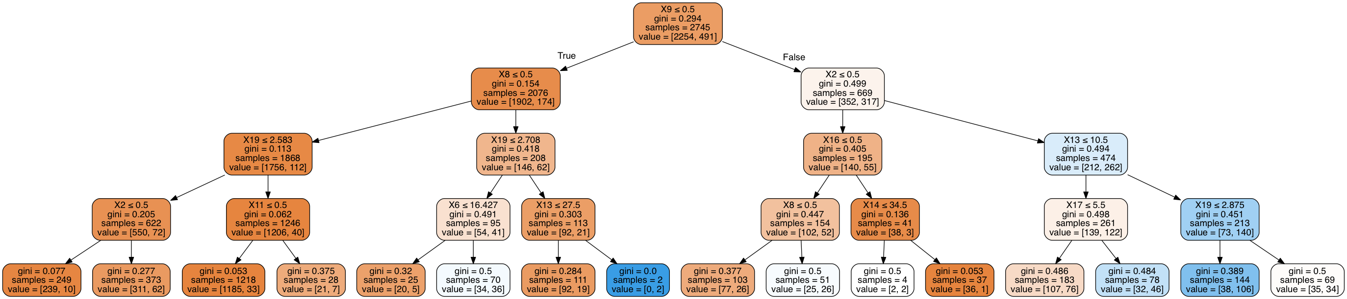
In [37]:
#Build model on training data
classifier=DecisionTreeClassifier(max_depth = 4)
classifier=classifier.fit(pred_train,tar_train)
predictions=classifier.predict(pred_test)

sklearn.metrics.confusion_matrix(tar_test,predictions)
Out[37]:
array([[1415,   99],
       [ 193,  123]])
In [38]:
sklearn.metrics.accuracy_score(tar_test, predictions)
Out[38]:
0.84043715846994538
In [39]:
from sklearn.externals.six import StringIO
from IPython.display import Image
from sklearn.tree import export_graphviz
import pydotplus
dot_data2 = StringIO()
export_graphviz(classifier, out_file=dot_data2,
                filled=True, rounded=True,
                special_characters=True)
graph2 = pydotplus.graph_from_dot_data(dot_data2.getvalue())
Image(graph2.create_png())
Out[39]:
In [40]:
sklearn.metrics.accuracy_score(tar_test, predictions)
Out[40]:
0.84043715846994538